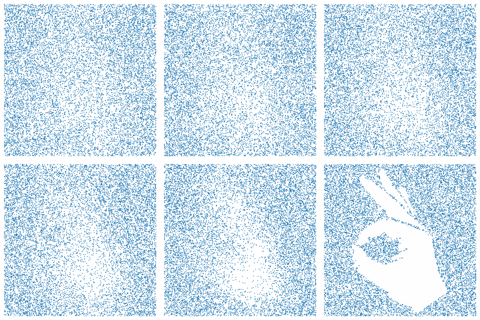
Diffusion drawing
Published:
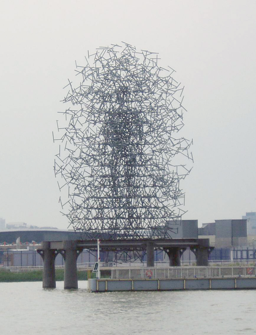
In London, there is a sculpture called Quantum Cloud, where the silhouette of a person emerges from a random walk of steel bars. Inspired by this idea, and bored during an A1 Swedish class, I wanted to replicate the effect and use random walks to create two-dimensional images.
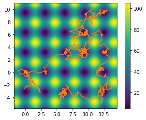
For simplicity, let’s focus on black-and-white images. One way to achieve contrast is to make the random walker spend more time in dark areas and less time in light areas. A two-dimensional walker with position-dependent drift and isotropic diffusivity may be simulated from the Langevin equation
In the absence of forcing ((\mathbf{A}=0)), this walker spends more time in regions where the diffusivity (D) is low, as illustrated in Fig. 2.
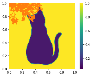
However, with this method, short trajectories typically do not have time to explore the full image, making it difficult to recognize, while long trajectories are too dense and lose any visual indication of randomness. I wanted a method that produced recognizable images while still “looking random.” To this end, I combined two kinds of motion: the walker takes Gaussian steps in dark pixels and Lévy-flight steps in light pixels. Because the Cauchy step-length distribution used for the Lévy flight is heavy-tailed, it occasionally produces very long jumps that make the trajectory look sparser. Fig. 3 shows the result: the cat’s geometry is much more visible, yet there is still some visual chaos and randomness. Varying the walker’s parameters produces different image textures.
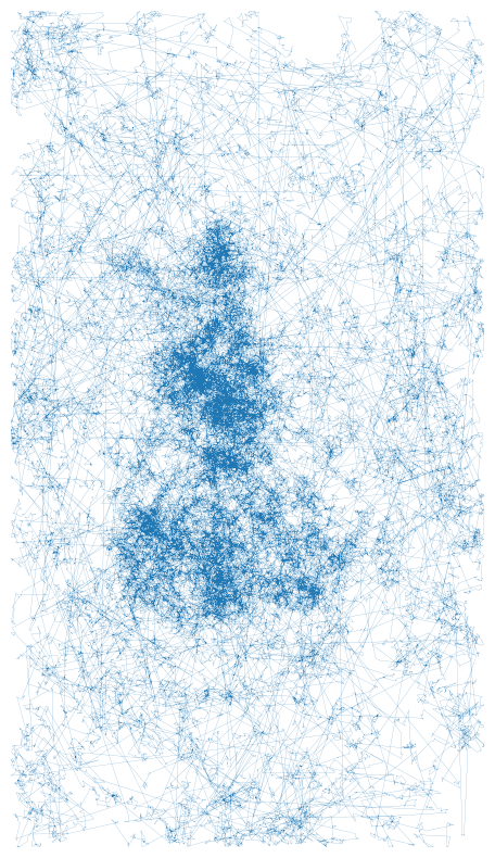
A simple way to extend this method from black-and-white to grayscale images is to interpret the pixel values as a spatially varying diffusivity. Interpolating those values defines a continuous diffusivity function. At each simulation step, pixels below mid-gray produce short Gaussian displacements, while pixels above mid-gray produce heavy-tailed Lévy-flight displacements whose scale depends on the local intensity. Dark regions therefore accumulate many short segments, while bright regions are crossed by sparse, long jumps. The results are shown in Fig. 4. Again, the large parameter space can produce a variety of visual results.
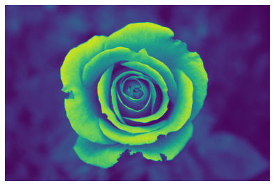
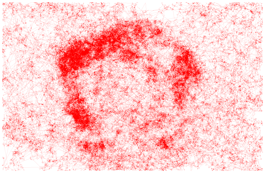
The result is less a conventional drawing algorithm than a way of encoding an image in the statistics of a path: local Gaussian motion supplies density, while Lévy flights supply negative space. It works best for images with strong tonal structure; fine details are lost, and the balance depends on the intensity threshold, step scale, and run length. Still, I like that the recognizable image is never drawn explicitly—it emerges from a single stochastic trajectory.