Replicating Wigner’s Insight

My friend Grigory Sarnitsky introduced me to experimental mathematics, where one uses guesswork to turn approximate but extensive computations into exact values or analytical insight. At first, I found the idea very unconvincing. Even after using it to compute infinite powers of large matrices for a paper, I remained a skeptic.

To give the idea a fair test, I wanted to reproduce a result where human guesswork played some role, and I decided on Wigner’s surmise. Could a computer rediscover it using Julia’s SymbolicRegression.jl?

What are we trying to rediscover?

Start with a large real symmetric matrix filled with random entries. Order its eigenvalues \(\lambda_k\) so that \(\lambda_1 < \lambda_2 < \dots\) and measure the gaps between neighbours. We will consider for the time being a small observation window, where the density of states does not change appreciably, but where we may still find many eigenvalues for a large matrix. We then consider the normalized gaps,

where \(\Delta\) is the local mean eigenvalue spacing. Thinking in terms of the normalized gaps removes the “uninteresting” effects of the density of states: obviously, if the density of states is higher the mean eigenvalue gap will be smaller.

For many kinds of random matrices, the normalized gaps follow universal laws determined by the symmetries of the ensemble. For Gaussian Orthogonal Ensembles (GOEs, defined below), the probability distribution of the local gap spacing is well-approximated by

Here, the probability density of a small gap vanishes linearly as \(s\to0\). This captures level repulsion: two eigenvalues in a GOE random matrix are unlikely to sit almost on top of each other. The Gaussian tail suppresses very large gaps. This expression is the famous Wigner surmise, introduced in 1956 during a conference to describe spacings between nuclear energy levels. This is the expression that we will try to reproduce from looking directly at eigenvalue data for large matrices.

Curiously, the law for the eigenvalue gap coincides with the one for a \(2\times 2\) GOE matrix, which can be derived analytically. I like the introduction in Embedded Random Matrix Ensembles in Quantum Physics by V.K.B. Kota if one just wants to read. The remarkable coincidence is that the same law also describes large matrices.

Sampling the GOE

The Gaussian orthogonal ensemble (GOE) consists of real symmetric \(N\times N\) matrices whose entries on and above the diagonal are independent Gaussian random variables with zero mean. We choose the off-diagonal entries to have variance \(1/N\) and the diagonal entries to have variance \(2/N\); the remaining entries are fixed by symmetry, \(H_{ji}=H_{ij}\). This normalization keeps the eigenvalues of order one as \(N\) grows. The code below samples this ensemble by generating ten \(5000\times5000\) matrices.

using LinearAlgebra
using Statistics

function GOE_matrix(N)
    A = randn(N, N)
    return (A + A') / sqrt(2)
end

N = 5000
ensemble_size = 10

matrix_ensemble = [GOE_matrix(N) / sqrt(N) for _ in 1:ensemble_size]
eigenvalue_ensemble = [sort(eigvals(M)) for M in matrix_ensemble]

Before looking at spacings, we may do a little sanity check by comparing the normalized eigenvalue distribution with the semicircle law (another universal law in random matrix theory, this time for the density of states)

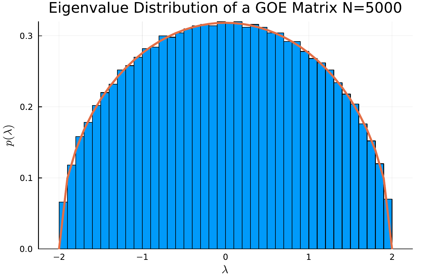
Spectral unfolding: dealing with a non-uniform density of states

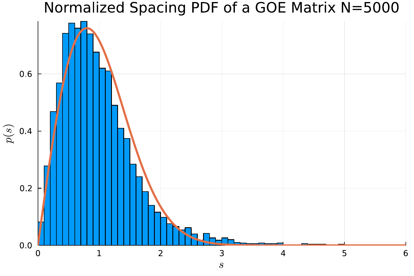
At this point one may get impatient, directly compute the eigenvalue gaps with diff(eigs), and divide all of them by one global mean.

spacings_ensemble = [diff(eigs) for eigs in eigenvalue_ensemble]
all_spacings = reduce(vcat, spacings_ensemble)
normalized_spacings = all_spacings / mean(all_spacings)

Unfortunately, this does not quite work, as Fig. 2 shows. The issue is that eigenvalues crowd together near the centre of the semicircle and spread out near its edges. This is simply a consequence of the varying density of states. The global mean then mixes regions with different local densities, leaving the visible disagreement below.

Fixing this local effect is one of the initially surprising points of random matrix theory (in my opinion). It is called spectral unfolding, and there are various ways of doing it depending on how good a handle we have on the behaviour of the eigenvalues. In this case, we have it easy because we know the limiting distribution law exactly. Indeed, we can then use the cumulative density of states

to unfold the eigenvalues according to

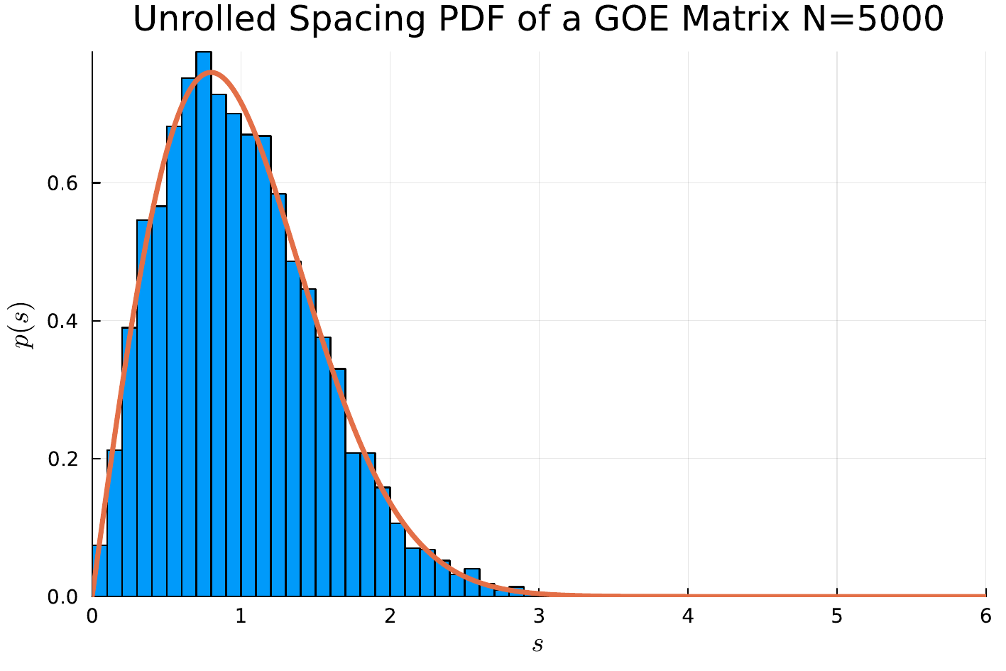
In other words, we replace each eigenvalue by the expected number of eigenvalues below it. Since \(dx=N\rho_{\mathrm{sc}}(\lambda)\,d\lambda\), an interval containing one eigenvalue on average becomes an interval of length one. Therefore, the unfolded spectrum has a constant unit local mean spacing, as we wanted.

function semicircle_cdf(x)
    if x <= -2 return 0 end
    if x >= 2 return 1 end
    return 1/2 +
        (x * sqrt(4 - x^2) + 4 * asin(x/2)) / (4π)
end

unfolded_ensemble = []
for eigs in eigenvalue_ensemble
    unfolded = [N * semicircle_cdf(λ) for λ in eigs]
    push!(unfolded_ensemble, unfolded)
end

spacings_ensemble = [diff(eigs) for eigs in unfolded_ensemble]
normalized_spacings = reduce(vcat, spacings_ensemble)

Recently, I found out a more direct way to approach this problem, which I believe it is not as mainstream as other unfolding methods. Since the issue is the differences in local density, consider the local gap ratio \(r_n = (\lambda_{n+1}-\lambda_n)/(\lambda_n-\lambda_{n-1})\). The idea is that the effects of the local density of states should cancel between denominator and numerator. The ratio distribution $P(r)$ is also known, so it is an alternative approach to the same universal properties. I found this out in Giraud et al., 2022, with the original reference being Oganesyan and Huse, 2007 I believe.

Let the computer guess

To use symbolic regression one needs functions: pairs of inputs and outputs. We must thus process the histogram data a bit, and I decided to smooth the unfolded data into a probability density using a Gaussian kernel-density estimate (KDE). Essentially, at each data point we place a Gaussian curve, where the width \(h\) of the Gaussian is the parameter controlling how much we are “smoothing” the function. For the spacing, I use Silverman’s rule, which seemed standard in the literature. This is a practical step, but not an innocent one. The regression will learn the KDE–an approximation built from a finite random sample–rather than Wigner’s formula itself.

function build_kde(data; bandwidth=nothing)
    n = length(data)

    if bandwidth === nothing
        μ = sum(data) / n
        σ = sqrt(sum((d - μ)^2 for d in data) / (n - 1))
        h = 1.06 * σ * n^(-1/5)
    else
        h = bandwidth
    end

    return function (x)
        total = sum(exp(-((x - d) / h)^2 / 2) for d in data)
        return total / (n * h * sqrt(2π))
    end
end

kde_pdf = build_kde(normalized_spacings)
x_vals = LinRange(0, 6, 1000)
y_vals = [kde_pdf(x) for x in x_vals]

Now for the actual symbolic regression part. The way the algorithm works is that, given a set of allowed operations (in our case the four arithmetic operations and exp), the code will combine them to create an analytical expression. It will then try to find the “best” combination, which both fits the data and is “not too complex” according to some parameters we can specify (such as how much recursion or how long we would like our expression to be). It does this through a genetic algorithm I believe, but the beauty of the Julia package is that all of the optimization is already implemented, and even without knowing any machine learning you can use it directly.

using SymbolicRegression
using MLJ

model = SRRegressor(
    binary_operators=[+, -, *, /],
    unary_operators=[exp],
    niterations=30,
)

mach = machine(model, [x_vals;;], y_vals)
fit!(mach)

r = report(mach)
r.equations[r.best_idx]

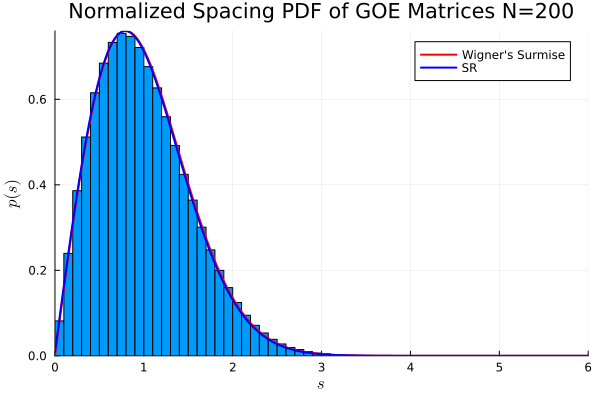
The output is a set of expressions that trade accuracy against complexity. Among the produced expressions, I found

Compare those numbers with \(\pi/2\approx1.57080\) and \(\pi/4\approx0.78540\). Very close! Moreover, the computer had recovered the important structure–a linear factor multiplied by a Gaussian in \(s^2\). Very cool! Another run found a slightly messier version:

The same pattern is hiding inside it. Rearranging the constant prefactor gives \(\exp(0.56698\times0.79503)\approx1.56952\), again very close to \(\pi/2\). The exponent, \(0.79503\), is still a little farther from \(\pi/4\).

At this point I was reasonably happy, but I think a lot of interesting questions remain open. For example, what if we have partial theoretical knowledge? For instance, some symmetry or asymptotic behaviour, how can we incorporate that? I tried to force \(p(0)=0\) by manually adding one hundred copies of \((0,0)\) to the data, which did result in analytical expressions where \(p(0)=0\), but is very inelegant. Probably such conditions can be directly implemented at the loss function level, but that remains for a future post.

So, did the computer rediscover Wigner’s insight? Not quite, since even if we were very sure of the expression, it proves nothing. However, organizing a cloud of numerical data into familiar analytical expressions is very useful for noticing patterns that can lead to true insight. If you thought the notion of symbolic regression is interesting, I recommend you check out the RIES algorithm and the discussion in their webpage, which is very interesting and clear.